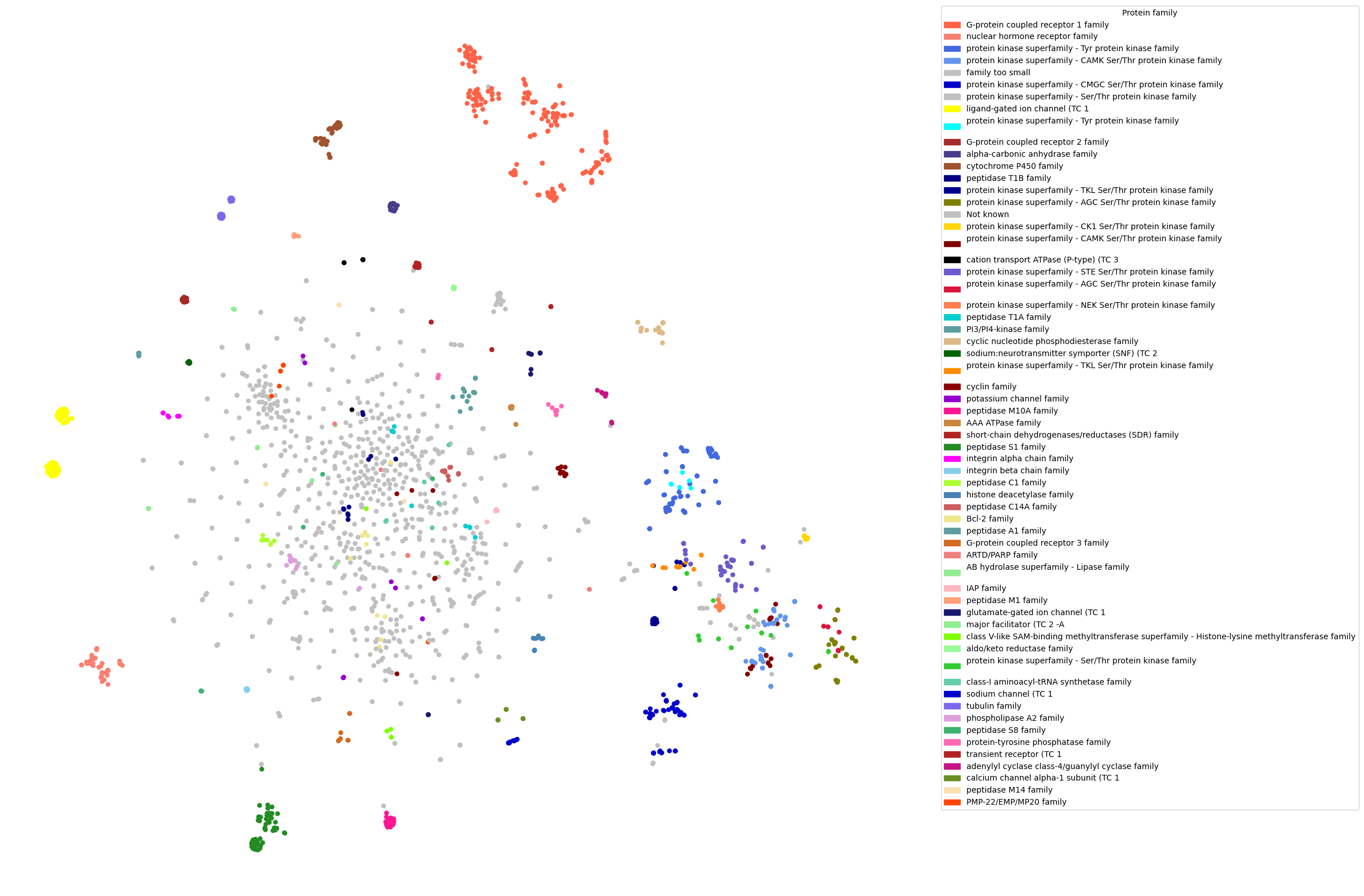
Visualization in the protein space

[2]:

%load_ext autoreload
%autoreload 2

import pandas as pd
import komet
import torch
import pickle
import numpy as np
import sklearn.manifold
import matplotlib.pyplot as plt

cpu

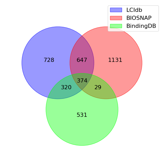
Comparison of the coverage of the protein space for LCIdb and other databases

1. Load datas

BindingDB dataset

[3]:

data_dir = './data/'
path_data_set = 'BindingDB'
dataset_dir = data_dir + path_data_set

# load data
train_BindingDB = komet.load_df("train.csv",dataset_dir)
val_BindingDB = komet.load_df("val.csv",dataset_dir)
test_BindingDB = komet.load_df( "test.csv",dataset_dir)

# dataframe full has all smiles and fasta sequences
full_BindingDB = pd.concat([train_BindingDB, val_BindingDB, test_BindingDB])
print("full shape",full_BindingDB.shape)
full_BindingDB.head()

number of smiles to clean: 0
train.csv shape (12668, 5)

[10:55:53] Explicit valence for atom # 22 N, 4, is greater than permitted
[10:55:53] Explicit valence for atom # 22 N, 4, is greater than permitted

number of smiles to clean: 2
val.csv shape (6642, 5)

[10:55:54] Explicit valence for atom # 22 N, 4, is greater than permitted
[10:55:54] Explicit valence for atom # 22 N, 4, is greater than permitted
[10:55:54] Explicit valence for atom # 22 N, 4, is greater than permitted

number of smiles to clean: 4
test.csv shape (13285, 5)
full shape (32595, 5)

[10:55:54] Can't kekulize mol.  Unkekulized atoms: 16 17 18 19 20 21 22 23 25

[3]:

	SMILES	Target Sequence	Label	drug_encoding	target_encoding
0	Cc1ccc(CNS(=O)(=O)c2ccc(s2)S(N)(=O)=O)cc1	MSHHWGYGKHNGPEHWHKDFPIAKGERQSPVDIDTHTAKYDPSLKP...	1	[0. 0. 0. ... 0. 0. 0.]	[5. 2.692 3.846 ... 0. 0. 0. ]
1	COc1ccc(CNS(=O)(=O)c2ccc(s2)S(N)(=O)=O)cc1	MSHHWGYGKHNGPEHWHKDFPIAKGERQSPVDIDTHTAKYDPSLKP...	1	[0. 0. 0. ... 0. 0. 0.]	[5. 2.692 3.846 ... 0. 0. 0. ]
2	NS(=O)(=O)c1ccc(s1)S(=O)(=O)NCc1cccs1	MSHHWGYGKHNGPEHWHKDFPIAKGERQSPVDIDTHTAKYDPSLKP...	1	[0. 0. 0. ... 0. 0. 0.]	[5. 2.692 3.846 ... 0. 0. 0. ]
3	NS(=O)(=O)c1cc2C(O)CN(Cc3cccs3)S(=O)(=O)c2s1	MSHHWGYGKHNGPEHWHKDFPIAKGERQSPVDIDTHTAKYDPSLKP...	1	[0. 0. 0. ... 0. 0. 0.]	[5. 2.692 3.846 ... 0. 0. 0. ]
4	COc1ccc(cc1)N1CC(O)c2cc(sc2S1(=O)=O)S(N)(=O)=O	MSHHWGYGKHNGPEHWHKDFPIAKGERQSPVDIDTHTAKYDPSLKP...	1	[0. 0. 0. ... 0. 0. 0.]	[5. 2.692 3.846 ... 0. 0. 0. ]

[4]:

# list of smiles
smiles_BindingDB = full_BindingDB[['SMILES']].drop_duplicates().values.flatten()
print("number of smiles",len(smiles_BindingDB))

# list of fasta sequences
fastas_BindingDB = full_BindingDB[['Target Sequence']].drop_duplicates().values.flatten()
print("number of sequences",len(fastas_BindingDB))

full_BindingDB[['Label']].value_counts()

number of smiles 7161
number of sequences 1254

[4]:

Label
0        23429
1         9166
dtype: int64

LCIdb dataset

[5]:

path_data_set = 'CC/full_data_S1'
dataset_dir = data_dir + path_data_set

# load data
train_LCIdb = komet.load_df("train.csv",dataset_dir)
val_LCIdb = komet.load_df("val.csv",dataset_dir)
test_LCIdb = komet.load_df( "test.csv",dataset_dir)

# dataframe full has all smiles and fasta sequences
full_LCIdb = pd.concat([train_LCIdb, val_LCIdb, test_LCIdb])
print("full shape",full_LCIdb.shape)
full_LCIdb.head()

number of smiles to clean: 0
train.csv shape (644060, 3)
number of smiles to clean: 0
val.csv shape (64408, 3)
number of smiles to clean: 0
test.csv shape (96608, 3)
full shape (805076, 3)

[5]:

	SMILES	Target Sequence	Label
0	NS(=O)(=O)c1ccc(CCNC(=S)N[C@@H]2O[C@H](CO)[C@@...	MSHHWGYGKHNGPEHWHKDFPIAKGERQSPVDIDTHTAKYDPSLKP...	1
1	NS(=O)(=O)c1ccc(CCNC(=S)N[C@@H]2O[C@H](CO)[C@@...	MQYLNIKEDCNAMAFCAKMRSSKKTEVNLEAPEPGVEVIFYLSDRE...	0
2	NS(=O)(=O)c1ccc(CCNC(=S)N[C@@H]2O[C@H](CO)[C@@...	MPPGVDCPMEFWTKEENQSVVVDFLLPTGVYLNFPVSRNANLSTIK...	0
3	NS(=O)(=O)c1ccc(CCNC(=S)N[C@@H]2O[C@H](CO)[C@@...	MASPDWGYDDKNGPEQWSKLYPIANGNNQSPVDIKTSETKHDTSLK...	1
4	NS(=O)(=O)c1ccc(CCNC(=S)N[C@@H]2O[C@H](CO)[C@@...	MLFSALLLEVIWILAADGGQHWTYEGPHGQDHWPASYPECGNNAQS...	1

[6]:

# list of smiles
smiles_LCIdb = full_LCIdb[['SMILES']].drop_duplicates().values.flatten()
print("number of smiles",len(smiles_LCIdb))

# list of fasta sequences
fastas_LCIdb = full_LCIdb[['Target Sequence']].drop_duplicates().values.flatten()
print("number of sequences",len(fastas_LCIdb))

full_LCIdb[['Label']].value_counts()

number of smiles 274515
number of sequences 2069

[6]:

Label
0        402538
1        402538
dtype: int64

Biosnap dataset

[7]:

path_data_set = 'BIOSNAP/full_data'
dataset_dir = data_dir + path_data_set

# load data
train_Biosnap = komet.load_df("train.csv",dataset_dir)
val_Biosnap = komet.load_df("val.csv",dataset_dir)
test_Biosnap = komet.load_df( "test.csv",dataset_dir)

# dataframe full has all smiles and fasta sequences
full_Biosnap = pd.concat([train_Biosnap, val_Biosnap, test_Biosnap])
print("full shape",full_Biosnap.shape)
full_Biosnap.head()

[10:57:22] Unusual charge on atom 0 number of radical electrons set to zero

number of smiles to clean: 0
train.csv shape (19238, 7)
number of smiles to clean: 0
val.csv shape (2748, 7)
number of smiles to clean: 0
test.csv shape (5497, 7)
full shape (27483, 7)

[10:57:23] Unusual charge on atom 0 number of radical electrons set to zero

[7]:

	Unnamed: 0	Unnamed: 0.1	DrugBank ID	Gene	Label	SMILES	Target Sequence
0	3	4	DB08533	P49862	0.0	CC1=CN=C2N1C=CN=C2NCC1=CC=NC=C1	MARSLLLPLQILLLSLALETAGEEAQGDKIIDGAPCARGSHPWQVA...
1	4	5	DB00755	P48443	1.0	C\C(\C=C\C1=C(C)CCCC1(C)C)=C/C=C/C(/C)=C/C(O)=O	MYGNYSHFMKFPAGYGGSPGHTGSTSMSPSAALSTGKPMDSHPSYT...
2	5	6	DB00361	O60218	0.0	[H][C@@]12N(C)C3=CC(OC)=C(C=C3[C@@]11CCN3CC=C[...	MATFVELSTKAKMPIVGLGTWKSPLGKVKEAVKVAIDAGYRHIDCA...
3	7	8	DB01136	P08588	1.0	COC1=CC=CC=C1OCCNCC(O)COC1=CC=CC2=C1C1=CC=CC=C1N2	MGAGVLVLGASEPGNLSSAAPLPDGAATAARLLVPASPPASLLPPA...
4	8	9	DB06963	Q9Y691	0.0	[H][C@@](C)(NC1=CC2=C(C=N1)C(C)=NN2C1=CC=CC(CC...	MFIWTSGRTSSSYRHDEKRNIYQKIRDHDLLDKRKTVTALKAGEDR...

[8]:

# list of smiles
smiles_Biosnap = full_Biosnap[['SMILES']].drop_duplicates().values.flatten()
print("number of smiles",len(smiles_Biosnap))

# list of fasta sequences
fastas_Biosnap = full_Biosnap[['Target Sequence']].drop_duplicates().values.flatten()
print("number of sequences",len(fastas_Biosnap))

full_Biosnap[['Label']].value_counts()

number of smiles 4510
number of sequences 2181

[8]:

Label
1.0      13836
0.0      13647
dtype: int64

2. Fastas

[9]:

L_prot_LCIdb = list(full_LCIdb["Target Sequence"].drop_duplicates())
L_prot_BindingDB_full = list(full_BindingDB["Target Sequence"].drop_duplicates())
L_prot_Biosnap = list(full_Biosnap["Target Sequence"].drop_duplicates())

L_prot_total = list( set(L_prot_LCIdb)  | set(L_prot_BindingDB_full) | set(L_prot_Biosnap))
print("nombre total de fasta",len(L_prot_total))

nombre total de fasta 3760

[10]:

L_fasta_total = L_prot_LCIdb +  L_prot_Biosnap + L_prot_BindingDB_full
print("nombre de fasta en concaténant les 3 listes",len(L_fasta_total))
nb_prot = len(L_fasta_total)

nombre de fasta en concaténant les 3 listes 5504

[11]:

from venn import venn
venn({'LCIdb': set(L_prot_LCIdb),  'BIOSNAP': set(L_prot_Biosnap), 'BindingDB': set(L_prot_BindingDB_full)}, cmap='brg', fontsize=16)

[11]:

<Axes: >

../_images/vignettes_Visualization_Proteins_16_1.png

3. Features with Uniprot LAkernel

[7]:

# Load Precomputed kernel and dict for the proteins
dict_ind2fasta_all = pickle.load(open(data_dir + "/dict_ind2fasta_all.data", 'rb'))
dict_fasta2ind_all = {fasta:ind for ind,fasta in dict_ind2fasta_all.items()}
U = torch.from_numpy(np.load(data_dir + "U_small.npy"))
Lambda = torch.from_numpy(np.load(data_dir + "Lambda_small.npy"))

#dict_ind2fasta_all = pickle.load(open("data/dict_ind2fasta_all.data", 'rb'))
#dict_fasta2ind_all = {fasta:ind for ind,fasta in dict_ind2fasta_all.items()}
#U = torch.from_numpy(np.load("data/U_small.npy"))
#Lambda = torch.from_numpy(np.load("data/Lambda_small.npy"))
print("U.shape",U.shape,"Lambda.shape",Lambda.shape)

U.shape torch.Size([20605, 1200]) Lambda.shape torch.Size([1200])

[8]:

# Load features for protein
dP = min(U.shape[0],1200)
Y_all = U[:,:dP] @ torch.diag(torch.sqrt(Lambda[:dP]))
Y_all = U[:,:dP] @ torch.diag(torch.sqrt(Lambda[:dP]))

# Protein kernel for the dataset
I_fasta = [dict_fasta2ind_all[L_fasta_total[i]] for i in range(len(L_fasta_total))] # index of fasta in the precomputed dict and protein kernel, in the same order as the dataset
Y = Y_all[I_fasta,:]
print("Y shape",Y.shape)

mytype=torch.float32
device = torch.device('cuda' if torch.cuda.is_available() else 'cpu')

Y = Y.to(device)
# nomramlisation of the features
Y_c = Y - Y.mean(axis = 0)
Y_cn = Y_c / torch.norm(Y_c,dim = 1)[:,None]

---------------------------------------------------------------------------
NameError                                 Traceback (most recent call last)
Cell In[8], line 7
      4 Y_all = U[:,:dP] @ torch.diag(torch.sqrt(Lambda[:dP]))
      6 # Protein kernel for the dataset
----> 7 I_fasta = [dict_fasta2ind_all[L_fasta_total[i]] for i in range(len(L_fasta_total))] # index of fasta in the precomputed dict and protein kernel, in the same order as the dataset
      8 Y = Y_all[I_fasta,:]
      9 print("Y shape",Y.shape)

NameError: name 'L_fasta_total' is not defined

4. Visualisation using T-SNE on different datasets

[14]:

# Visualisation using T-SNE

perp = 50 # increase for less randomness
Y_T = sklearn.manifold.TSNE(n_components=2, perplexity=perp).fit_transform(Y_cn.numpy())

[15]:

import matplotlib.patches as mpatches

n_LCIdb = len(L_prot_LCIdb)
n_Biosnap = len(L_prot_Biosnap)
n_BindingDB_full = len(L_prot_BindingDB_full)

plt.rc('font', family="Times New Roman")
plt.rc('text', usetex=True)

# faire 3 figures cote à cote
fig, axes = plt.subplots(1, 3, figsize=(9, 3))
axes[0].scatter(Y_T[:n_LCIdb,0], Y_T[:n_LCIdb,1],c = 'blue',s=1,label = 'LCIdb proteins');
axes[0].set_title(r'LCIdb',fontsize=20)
axes[0].axis('off')


axes[1].scatter(Y_T[:n_LCIdb,0], Y_T[:n_LCIdb,1],c = 'blue',s=3,label = 'prot in LCIdb');
axes[1].scatter(Y_T[(n_LCIdb):(n_LCIdb+n_Biosnap),0], Y_T[(n_LCIdb):(n_LCIdb+n_Biosnap),1],c = 'r',s=1,label = 'prot in Biosnap');
axes[1].axis('off')
axes[1].set_title(r'BIOSNAP',fontsize=20)

axes[2].scatter(Y_T[:n_LCIdb,0], Y_T[:n_LCIdb,1],c = 'blue',s=3,label = 'prot in LCIdb');
axes[2].scatter(Y_T[(n_LCIdb+n_Biosnap):,0], Y_T[(n_LCIdb+n_Biosnap):,1],c = 'r',s=1,label = 'prot in BindingDB');
axes[2].axis('off')
axes[2].set_title(r'BindingDB',fontsize=20)

# titre
plt.suptitle("t-SNE visualization on LAkernel features", fontsize=16, y=0.05)


plt.show()

../_images/vignettes_Visualization_Proteins_22_0.png

Visualisation using T-SNE on different proteins family on LCIdb

[3]:

# add uniprot id to the dataframe
LCIdb = pd.read_csv(data_dir + "LCIdb.csv") # load the dataframe from Zenodo
LCIdb.head()

[3]:

	smiles	fasta	ChEMBL ID	PubChem ID	IUPHAR ID	Ligand names	Target	uniprot	mean	mean pIC50	...	min pIC50	min pKi	min pKd	max	max pIC50	max pKi	max pKd	score	indsmiles	indfasta
0	BrC1CCN(Cc2ccc(OCCCN3CCCCC3)cc2)CC1	MERAPPDGPLNASGALAGEAAAAGGARGFSAAWTAVLAALMALLIV...	CHEMBL472466	44592131.0	NaN	4-bromo-1-(4-(3-(piperidin-1-yl)propoxy)benzyl...	hrh3	Q9Y5N1	9.7	NaN	...	NaN	9.7	NaN	9.7	NaN	9.7	NaN	1.0	0.0	0.0
1	BrCC(Br)C1CCC(Br)C(Br)C1	MEVQLGLGRVYPRPPSKTYRGAFQNLFQSVREVIQNPGPRHPEAAS...	CHEMBL375107	18728.0	NaN	1,2-dibromo-4-(1,2-dibromoethyl)cyclohexane\nn...	ar	P10275	7.4	7.4	...	7.4	NaN	NaN	7.4	7.4	NaN	NaN	1.0	1.0	1.0
2	BrC[C@H]1CC[C@H](c2nnn3cnc4[nH]ccc4c23)CC1	MAPPSEETPLIPQRSCSLLSTEAGALHVLLPARGPGPPQRLSFSFG...	CHEMBL3918308	136641870.0	NaN	us9216999, 74	jak3	P52333	7.1	7.1	...	7.1	NaN	NaN	7.1	7.1	NaN	NaN	1.0	2.0	2.0
3	BrC[C@H]1CC[C@H](c2nnn3cnc4[nH]ccc4c23)CC1	MGMACLTMTEMEGTSTSSIYQNGDISGNANSMKQIDPVLQVYLYHS...	CHEMBL3918308	136641870.0	NaN	us9216999, 74	jak2	O60674	8.5	8.5	...	8.5	NaN	NaN	8.5	8.5	NaN	NaN	1.0	2.0	3.0
4	BrC[C@H]1CC[C@H](c2nnn3cnc4[nH]ccc4c23)CC1	MPLRHWGMARGSKPVGDGAQPMAAMGGLKVLLHWAGPGGGEPWVTF...	CHEMBL3918308	136641870.0	NaN	us9216999, 74	tyk2	P29597	8.6	8.6	...	8.6	NaN	NaN	8.6	8.6	NaN	NaN	1.0	2.0	4.0

5 rows × 23 columns

[18]:

df_prot_LCIdb = LCIdb[['uniprot',"fasta"]].drop_duplicates()
df_prot_LCIdb.shape

[18]:

(2071, 2)

[20]:

L_prot_LCIdb = list(df_prot_LCIdb["fasta"])
len(L_prot_LCIdb)

[20]:

The file similar.txt is available at https://www.uniprot.org/ There is a new Swiss-Prot document: similar.txt : Index of CC SIMILARITY lines. This index lists all names of families and domains occurring in CC SIMILARITY lines of Swiss-Prot entries.

[21]:

def f(x):
    if "family" in x:
        if "superfamily" in x:
            try:
                return x.split(".")[0] +" -"+ x.split(".")[1]
            except :
                return x
            #return x.split(".")[0] +" -"+ x.split(".")[1]
        if "subfamily" in x:
            return x.split(".")[0]
        #if "peptidase" in x:
        #    return "peptidase family"
        #if "SAM-binding methyltransferase superfamily" in x:
        #    return "SAM-binding methyltransferase superfamily"
        else:
            return x.strip('\n')
    else:
        return x


def find_family(uniprot_id):
    file_path = './data/similar.txt'
    with open(file_path, 'r') as file:
        lines = file.readlines()

    family_dict = {}
    current_family = None
    list_uniprots = []

    for line in lines:
        # Check if the line contains the word 'family'
        if 'family' in line:
            current_family = line

        elif '(' in line:
            #If the line contains a parentheses, it could contain UniProts in parentheses
            parts = line.split(',')
            parts = [part.strip() for part in parts]
            parts = [part.strip('()')[-6:] for part in parts]
            if uniprot_id in parts:
                return f(current_family)

    # If UniProt is not found
    return "Not known"

[22]:

df_prot_LCIdb["family"] = df_prot_LCIdb["uniprot"].apply(lambda x: find_family(x))
df_prot_LCIdb["family"].value_counts()

[22]:

G-protein coupled receptor 1 family                                181
Not known                                                          154
protein kinase superfamily - Tyr protein kinase family              75
protein kinase superfamily - CMGC Ser/Thr protein kinase family     50
peptidase S1 family                                                 47
                                                                  ...
ADRM1 family                                                         1
DSS1/SEM1 family                                                     1
proteasome subunit S10 family                                        1
proteasome subunit S3 family                                         1
camello family                                                       1
Name: family, Length: 565, dtype: int64

[23]:

df_family = pd.DataFrame(df_prot_LCIdb["family"].value_counts())
# change the index to a column named family
df_family.reset_index(inplace=True)
df_family.columns = ["family","count"]
#df_family[df_family["count"] > 5]
# to make the color, I add a column with None if count < 10
df_prot_LCIdb["family_2"] = df_prot_LCIdb["family"].apply(lambda x: x if x in df_family[df_family["count"] > 5]["family"].to_list() else "family too small")
df_prot_LCIdb["family_2"].value_counts()

[23]:

family too small                                                   793
G-protein coupled receptor 1 family                                181
Not known                                                          154
protein kinase superfamily - Tyr protein kinase family              75
protein kinase superfamily - CMGC Ser/Thr protein kinase family     50
                                                                  ...
class-I aminoacyl-tRNA synthetase family                             7
ARTD/PARP family                                                     7
aldo/keto reductase family                                           7
major facilitator (TC 2 -A                                           6
IAP family                                                           6
Name: family_2, Length: 61, dtype: int64

[29]:

# Protein kernel for the dataset
I_fasta_LCIdb = [dict_fasta2ind_all[L_prot_LCIdb[i]] for i in range(len(L_prot_LCIdb))] # index of fasta in the precomputed dict and protein kernel, in the same order as the dataset
Y_LCIdb = Y_all[I_fasta_LCIdb,:]
print("Y shape",Y_LCIdb.shape)

mytype=torch.float32
device = torch.device('cuda' if torch.cuda.is_available() else 'cpu')

Y_LCIdb = Y_LCIdb.to(device)
# nomramlisation of the features
Y_LCIdb_c = Y_LCIdb - Y_LCIdb.mean(axis = 0)
Y_LCIdb_cn = Y_LCIdb_c / torch.norm(Y_LCIdb_c,dim = 1)[:,None]

# Visualisation using T-SNE
perp = 30 # increase for less randomness
Y_LCIdb_T = sklearn.manifold.TSNE(n_components=2, perplexity=perp).fit_transform(Y_LCIdb_cn.numpy())

Y shape torch.Size([2071, 1200])

[36]:

import matplotlib.pyplot as plt
import matplotlib.patches as mpatches


fig, ax = plt.subplots(figsize=(20, 20))

# Define the matching dictionary between family_2 and colors
list_colors = ["tomato","salmon","royalblue","cornflowerblue","silver","mediumblue","silver","yellow","cyan","brown","darkslateblue","sienna","navy","darkblue","olive","silver","gold","maroon","black","slateblue","crimson","coral","darkturquoise","cadetblue","burlywood","darkgreen","darkorange","darkred","darkviolet","deeppink","peru","firebrick","forestgreen","fuchsia","skyblue","greenyellow","steelblue","indianred","khaki","cadetblue","chocolate","lightcoral","lightgreen","lightpink","lightsalmon","midnightblue","lightgreen","chartreuse","palegreen","limegreen","mediumaquamarine","mediumblue","mediumslateblue","plum","mediumseagreen","hotpink","firebrick","mediumvioletred","olivedrab","navajowhite","orangered","orchid","palegreen","paleturquoise","palevioletred","peru","plum","powderblue","rosybrown","royalblue","saddlebrown","salmon","sandybrown","seagreen","sienna","skyblue","slateblue","slategray","springgreen","steelblue","tan","thistle","tomato","turquoise","violet","wheat","silver"]
color_mapping = dict(zip(df_prot_LCIdb["family_2"].drop_duplicates(),list_colors))

# Utiliser le mapping pour obtenir les couleurs correspondantes à chaque famille
colors = df_prot_LCIdb["family_2"].map(color_mapping)

# Tracer les points en utilisant les couleurs
scatter = ax.scatter(x=Y_LCIdb_T [:, 0], y=Y_LCIdb_T [:, 1], c=colors, s=25)

# Créer une légende personnalisée avec les couleurs spécifiées
legend_patches = [mpatches.Patch(color=color_mapping[key], label=key) for key in color_mapping]
ax.legend(handles=legend_patches, title="Protein family", bbox_to_anchor=(1.05, 1), loc=2, borderaxespad=0.0)

ax.axis('off')

#plt.savefig("/Users/gguichaoua/Dropbox/gwenn/these/chemogenomique/Databases/databases_comparison/prot_cluster.pdf")
# Afficher le nuage de points
plt.show()

../_images/vignettes_Visualization_Proteins_32_0.png